Tutorial: Functions on LCAs

This is an interactive tutorial written with real code. We start by setting up \(\LaTeX\) printing, and importing the classes LCA, HomLCA and LCAFunc.

# Imports from abelian
from abelian import LCA, HomLCA, LCAFunc

# Other imports
import math
import matplotlib.pyplot as plt
from IPython.display import display, Math

def show(arg):
    return display(Math(arg.to_latex()))

Initializing a new function

There are two ways to create a function \(f: G \to \mathbb{C}\):

• On general LCAs \(G\), the function is represented by an analytical expression.
• If \(G = \mathbb{Z}_{\mathbf{p}}\) with \(p_i \geq 1\) for every \(i\) (\(G\) is a direct sum of discrete groups with finite period), a table of values (multidimensional array) can also be used.

With an analytical representation

If the representation of the function is given by an analytical expression, initialization is simple.

Below we define a Gaussian function on \(\mathbb{Z}\), and one on \(T\).

def gaussian(vector_arg, k = 0.1):
    return math.exp(-sum(i**2 for i in vector_arg)*k)

# Gaussian function on Z
Z = LCA([0])
gauss_on_Z = LCAFunc(gaussian, domain = Z)
print(gauss_on_Z) # Printing
show(gauss_on_Z) # LaTeX output

# Gaussian function on T
T = LCA([1], [False])
gauss_on_T = LCAFunc(gaussian, domain = T)
show(gauss_on_T) # LaTeX output

LCAFunc on domain [Z]

$$\operatorname{function} \in \mathbb{C}^G, \ G = \mathbb{Z}$$

$$\operatorname{function} \in \mathbb{C}^G, \ G = T$$

Notice how the print built-in and the to_latex() method will show human-readable output.

With a table of values

Functions on \(\mathbb{Z}_\mathbf{p}\) can be defined using a table of values, if \(p_i \geq 1\) for every \(p_i \in \mathbf{p}\).

# Create a table of values
table_data = [[1,2,3,4,5],
              [2,3,4,5,6],
              [3,4,5,6,7]]

# Create a domain matching the table
domain = LCA([3, 5])

table_func = LCAFunc(table_data, domain)
show(table_func)
print(table_func([1, 1])) # [1, 1] maps to 3

$$\operatorname{function} \in \mathbb{C}^G, \ G = \mathbb{Z}_{3} \oplus \mathbb{Z}_{5}$$

3

Function evaluation

A function \(f \in \mathbb{C}^G\) is callable. To call (i.e. evaluate) a function, pass a group element.

# An element in Z
element = [0]

# Evaluate the function
gauss_on_Z(element)

1.0

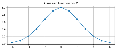
The sample() method can be used to sample a function on a list of group elements in the domain.

# Create a list of sample points [-6, ..., 6]
sample_points = [[i] for i in range(-6, 7)]

# Sample the function, returns a list of values
sampled_func = gauss_on_Z.sample(sample_points)

# Plot the result of sampling the function
plt.figure(figsize = (8, 3))
plt.title('Gaussian function on $\mathbb{Z}$')
plt.plot(sample_points, sampled_func, '-o')
plt.grid(True)
plt.show()

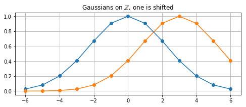
Shifts

Let \(f: G \to \mathbb{C}\) be a function. The shift operator (or translation operator) \(S_{h}\) is defined as

\[S_{h}[f(g)] = f(g - h).\]

The shift operator shifts \(f(g)\) by \(h\), where \(h, g \in G\).

The shift operator is implemented as a method called shift.

# The group element to shift by
shift_by = [3]

# Shift the function
shifted_gauss = gauss_on_Z.shift(shift_by)

# Create sample poits and sample
sample_points = [[i] for i in range(-6, 7)]
sampled1 = gauss_on_Z.sample(sample_points)
sampled2 = shifted_gauss.sample(sample_points)

# Create a plot
plt.figure(figsize = (8, 3))
ttl = 'Gaussians on $\mathbb{Z}$, one is shifted'
plt.title(ttl)
plt.plot(sample_points, sampled1, '-o')
plt.plot(sample_points, sampled2, '-o')
plt.grid(True)
plt.show()

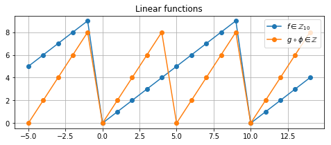
Pullbacks

Let \(\phi: G \to H\) be a homomorphism and let \(f:H \to \mathbb{C}\) be a function. The pullback of \(f\) along \(\phi\), denoted \(\phi^*(f)\), is defined as

\[\phi^*(f) := f \circ \phi.\]

The pullback “moves” the domain of the function \(f\) to \(G\), i.e. \(\phi^*(f) : G \to \mathbb{C}\). The pullback is of f is calculated using the pullback method, as shown below.

def linear(arg):
    return sum(arg)

# The original function
f = LCAFunc(linear, LCA([10]))
show(f)

# A homomorphism phi
phi = HomLCA([2], target = [10])
show(phi)

# The pullback of f along phi
g = f.pullback(phi)
show(g)

$$\operatorname{function} \in \mathbb{C}^G, \ G = \mathbb{Z}_{10}$$

$$\begin{pmatrix}2\end{pmatrix}:\mathbb{Z} \to \mathbb{Z}_{10}$$

$$\operatorname{function} \in \mathbb{C}^G, \ G = \mathbb{Z}$$

We now sample the functions and plot them.

# Sample the functions and plot them
sample_points = [[i] for i in range(-5, 15)]
f_sampled = f.sample(sample_points)
g_sampled = g.sample(sample_points)

# Plot the original function and the pullback
plt.figure(figsize = (8, 3))
plt.title('Linear functions')
label = '$f \in \mathbb{Z}_{10}$'
plt.plot(sample_points, f_sampled, '-o', label = label)
label = '$g \circ \phi \in \mathbb{Z}$'
plt.plot(sample_points, g_sampled, '-o', label = label)
plt.grid(True)
plt.legend(loc = 'best')
plt.show()

Pushforwards

Let \(\phi: G \to H\) be a epimorphism and let \(f:G \to \mathbb{C}\) be a function. The pushforward of \(f\) along \(\phi\), denoted \(\phi_*(f)\), is defined as

\[(\phi_*(f))(g) := \sum_{k \in \operatorname{ker}\phi} f(k + h), \quad \phi(g) = h\]

The pullback “moves” the domain of the function \(f\) to \(H\), i.e. \(\phi_*(f) : H \to \mathbb{C}\). First a solution is obtained, then we sum over the kernel. Since such a sum may contain an infinite number of terms, we bound it using a norm. Below is an example where we:

• Define a Gaussian \(f(x) = \exp(-kx^2)\) on \(\mathbb{Z}\)
• Use pushforward to “move” it with \(\phi(g) = g \in \operatorname{Hom}(\mathbb{Z}, \mathbb{Z}_{10})\)

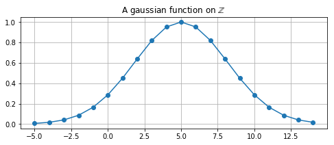
# We create a function on Z and plot it
def gaussian(arg, k = 0.05):
    """
    A gaussian function.
    """
    return math.exp(-sum(i**2 for i in arg)*k)

# Create gaussian on Z, shift it by 5
gauss_on_Z = LCAFunc(gaussian, LCA([0]))
gauss_on_Z = gauss_on_Z.shift([5])

# Sample points and sampled function
s_points = [[i] for i in range(-5, 15)]
f_sampled = gauss_on_Z.sample(s_points)

# Plot it
plt.figure(figsize = (8, 3))
plt.title('A gaussian function on $\mathbb{Z}$')
plt.plot(s_points, f_sampled, '-o')
plt.grid(True)
plt.show()

# Use a pushforward to periodize the function
phi = HomLCA([1], target = [10])
show(phi)

$$\begin{pmatrix}1\end{pmatrix}:\mathbb{Z} \to \mathbb{Z}_{10}$$

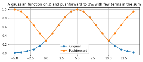
First we do a pushforward with only one term. Not enough terms are present in the sum to capture what the pushforward would look like if the sum went to infinity.

terms = 1

# Pushforward of the function along phi
gauss_on_Z_10 = gauss_on_Z.pushforward(phi, terms)

# Sample the functions and plot them
pushforward_sampled = gauss_on_Z_10.sample(sample_points)

plt.figure(figsize = (8, 3))
label = 'A gaussian function on $\mathbb{Z}$ and \
pushforward to $\mathbb{Z}_{10}$ with few terms in the sum'
plt.title(label)
plt.plot(s_points, f_sampled, '-o', label ='Original')
plt.plot(s_points, pushforward_sampled, '-o', label ='Pushforward')
plt.legend(loc = 'best')
plt.grid(True)
plt.show()

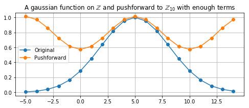
Next we do a pushforward with more terms in the sum, this captures what the pushforward would look like if the sum went to infinity.

terms = 9

gauss_on_Z_10 = gauss_on_Z.pushforward(phi, terms)

# Sample the functions and plot them
pushforward_sampled = gauss_on_Z_10.sample(sample_points)

plt.figure(figsize = (8, 3))
plt.title('A gaussian function on $\mathbb{Z}$ and \
pushforward to $\mathbb{Z}_{10}$ with enough terms')
plt.plot(s_points, f_sampled, '-o', label ='Original')
plt.plot(s_points, pushforward_sampled, '-o', label ='Pushforward')
plt.legend(loc = 'best')
plt.grid(True)
plt.show()